Векторное пространство

Algebraic structure in linear algebra

Сложение векторов и скалярное умножение: вектор v (синий) добавляется к другому вектору w (красный, верхний рисунок). Ниже w растянуто в 2 раза, что дает сумму v + 2 w .

В математике и физике векторное пространство (также называемое линейным пространством ) — это набор , элементы которого, часто называемые векторами , могут складываться вместе и умножаться («масштабироваться») на числа, называемые скалярами . Скаляры часто являются действительными числами , но могут быть и комплексными числами или, в более общем плане, элементами любого поля . Операции сложения векторов и скалярного умножения должны удовлетворять определенным требованиям, называемым векторными аксиомами . Действительные векторные пространства и комплексные векторные пространства — это виды векторных пространств, основанные на различных видах скаляров: действительных и комплексных числах .

Векторные пространства обобщают евклидовы векторы , которые позволяют моделировать физические величины , такие как силы и скорость , которые имеют не только величину , но и направление . Концепция векторных пространств является фундаментальной для линейной алгебры вместе с концепцией матриц , которая позволяет выполнять вычисления в векторных пространствах. Это обеспечивает краткий и синтетический способ манипулирования и изучения систем линейных уравнений .

Векторные пространства характеризуются своей размерностью , которая, грубо говоря, задает количество независимых направлений в пространстве. Это означает, что для двух векторных пространств над данным полем и одинаковой размерности свойства, которые зависят только от структуры векторного пространства, совершенно одинаковы (технически векторные пространства изоморфны ) . Векторное пространство является конечномерным, если его размерность является натуральным числом . В противном случае оно бесконечномерно , а его размерность — бесконечный кардинал . Конечномерные векторные пространства естественным образом встречаются в геометрии и смежных областях. Бесконечномерные векторные пространства встречаются во многих областях математики. Например, кольца полиномов представляют собой счетно -бесконечномерные векторные пространства, а многие функциональные пространства имеют мощность континуума в качестве размерности.

Многие векторные пространства, рассматриваемые в математике, наделены и другими структурами . Это случай алгебр , которые включают расширения полей , кольца многочленов, ассоциативные алгебры и алгебры Ли . Это также относится к топологическим векторным пространствам , которые включают функциональные пространства, пространства внутреннего произведения , нормированные пространства , гильбертовы пространства и банаховы пространства .

Определение и основные свойства

В этой статье векторы выделены жирным шрифтом, чтобы отличить их от скаляров. ^{[номер 1] [1]}

Векторное пространство над полем F — это непустое множество  V вместе с бинарной операцией и бинарной функцией , которые удовлетворяют восьми аксиомам, перечисленным ниже. В этом контексте элементы V обычно называются векторами , а элементы  F называются скалярами . ^[2]

• Бинарная операция, называемая сложением векторов или просто сложением , присваивает любым двум векторам  v и w в V третий вектор из V , который обычно записывается как v + w и называется суммой этих двух векторов.

• Бинарная функция, называемая скалярным умножением , присваивает любому скаляру  a из F и любому вектору  v из V другой вектор из V , который обозначается  как v . ^{[номер 2]}

Чтобы иметь векторное пространство, восемь следующих аксиом должны выполняться для всех u , v и w в V , а также a и b в F. ^[3]

Когда скалярное поле представляет собой действительные числа , векторное пространство называется действительным векторным пространством , а когда скалярное поле представляет собой комплексные числа , векторное пространство называется комплексным векторным пространством . ^[4] Эти два случая являются наиболее распространенными, но также часто рассматриваются векторные пространства со скалярами в произвольном поле F. Такое векторное пространство называется F - векторным пространством или векторным пространством над F. ^[5]

Можно дать эквивалентное определение векторного пространства, которое гораздо более краткое, но менее элементарное: первые четыре аксиомы (относящиеся к сложению векторов) говорят, что векторное пространство представляет собой абелеву группу при сложении, а четыре оставшиеся аксиомы (относящиеся к сложению векторов ) скалярное умножение) говорят, что эта операция определяет гомоморфизм колец из поля F в кольцо эндоморфизмов этой группы. ^[6]

Вычитание двух векторов можно определить как $${\displaystyle \mathbf {v} -\mathbf {w} =\mathbf {v} +(-\mathbf {w} ).}$$

Прямые следствия аксиом заключаются в том, что, поскольку каждый имеет ${\displaystyle s\in F}$ ${\displaystyle \mathbf {v} \in V,}$

• ${\displaystyle 0\mathbf {v} =\mathbf {0} ,}$
• ${\displaystyle s\mathbf {0} =\mathbf {0} ,}$
• ${\displaystyle (-1)\mathbf {v} =-\mathbf {v} ,}$
• ${\displaystyle s\mathbf {v} =\mathbf {0} }$подразумевает или ${\displaystyle s=0}$ ${\displaystyle \mathbf {v} =\mathbf {0} .}$

Если говорить еще более кратко, векторное пространство — это модуль над полем . ^[7]

Базисы, векторные координаты и подпространства

Вектор v в R ^{2 (синий)} , выраженный в различных базисах: с использованием стандартного базиса R ² : v = x e ₁ + y e ₂ (черный) и с использованием другого, неортогонального базиса : v = f ₁ + f ₂ (красный).

Линейная комбинация

Учитывая набор G элементов F -векторного пространства V , линейная комбинация элементов G представляет собой элемент V вида где и Скаляры называются коэффициентами линейной комбинации. ^[8] $${\displaystyle a_{1}\mathbf {g} _{1}+a_{2}\mathbf {g} _{2}+\cdots +a_{k}\mathbf {g} _{k},}$$ ${\displaystyle a_{1},\ldots ,a_{k}\in F}$ ${\displaystyle \mathbf {g} _{1},\ldots ,\mathbf {g} _{k}\in G.}$ ${\displaystyle a_{1},\ldots ,a_{k}}$

Линейная независимость

Элементы подмножества G F - векторного пространства V называются линейно независимыми , если ни один элемент G не может быть записан как линейная комбинация других элементов G . Эквивалентно, они линейно независимы, если две линейные комбинации элементов G определяют один и тот же элемент V тогда и только тогда, когда они имеют одинаковые коэффициенты. Аналогичным образом, они линейно независимы, если линейная комбинация приводит к нулевому вектору тогда и только тогда, когда все его коэффициенты равны нулю. ^[9]

Линейное подпространство

Линейное подпространство или векторное подпространство W векторного пространства V — это непустое подмножество V , замкнутое относительно векторного сложения и скалярного умножения; то есть сумма двух элементов W и произведение элемента W на скаляр принадлежат W . ^[10] Это означает, что каждая линейная комбинация элементов W принадлежит W . Линейное подпространство — это векторное пространство для индуцированного сложения и скалярного умножения; это означает, что свойство замыкания подразумевает, что аксиомы векторного пространства выполняются. ^[11]
Свойство замыкания также подразумевает, что каждое пересечение линейных подпространств является линейным подпространством. ^[11]

Линейный пролет

Учитывая подмножество G векторного пространства V , линейная оболочка или просто оболочка G является наименьшим линейным подпространством V , которое содержит G , в том смысле , что это пересечение всех линейных подпространств, содержащих G. Пространство G также является множеством всех линейных комбинаций элементов G . Если W является промежутком G , говорят, что G охватывает или порождает W и что G является охватывающим множеством или порождающим набором W. ^[12]

Основа и размерность

Подмножество векторного пространства является базисом , если его элементы линейно независимы и охватывают векторное пространство. ^[13] Каждое векторное пространство имеет по крайней мере один базис или вообще много (см. Базис (линейная алгебра) § Доказательство того, что каждое векторное пространство имеет базис ). ^[14] Более того, все базы векторного пространства имеют одинаковую мощность , которая называется размерностью векторного пространства (см. Теорему о размерности для векторных пространств ). ^[15] Это фундаментальное свойство векторных пространств, которое подробно описано в оставшейся части раздела.

Базисы — фундаментальный инструмент для изучения векторных пространств, особенно когда размерность конечна. В бесконечномерном случае существование бесконечных базисов, часто называемых базисами Гамеля , зависит от выбранной аксиомы . Отсюда следует, что, вообще говоря, ни одна база не может быть описана явно. ^[16] Например, действительные числа образуют бесконечномерное векторное пространство над рациональными числами , для которого неизвестен конкретный базис.

Рассмотрим базис векторного пространства V размерности n над полем F . Определение базиса подразумевает, что каждый может быть записан с в F и что это разложение уникально. Скаляры называются координатами v на базисе . Их также называют коэффициентами разложения v по базису. Также говорят, что n - кортеж координат является координатным вектором v на базисе, поскольку набор n - кортежей элементов F представляет собой векторное пространство для покомпонентного сложения и скалярного умножения, размерность которого равна n . ${\displaystyle (\mathbf {b} _{1},\mathbf {b} _{2},\ldots ,\mathbf {b} _{n})}$ ${\displaystyle \mathbf {v} \in V}$ $${\displaystyle \mathbf {v} =a_{1}\mathbf {b} _{1}+\cdots +a_{n}\mathbf {b} _{n},}$$ ${\displaystyle a_{1},\dots ,a_{n}}$ ${\displaystyle a_{1},\ldots ,a_{n}}$ ${\displaystyle F^{n}}$

Соответствие «один к одному» между векторами и их координатными векторами отображает сложение векторов в сложение векторов, а скалярное умножение — в скалярное умножение. Таким образом, это изоморфизм векторного пространства , который позволяет переводить рассуждения и вычисления над векторами в рассуждения и вычисления над их координатами. ^[17]

История

Векторные пространства происходят из аффинной геометрии путем введения координат в плоском или трехмерном пространстве. Около 1636 года французские математики Рене Декарт и Пьер де Ферма основали аналитическую геометрию , находя решения уравнения двух переменных с точками на плоской кривой . ^[18] Для достижения геометрических решений без использования координат Больцано ввел в 1804 году определенные операции над точками, линиями и плоскостями, которые являются предшественниками векторов. ^[19] Мёбиус (1827) ввёл понятие барицентрических координат . ^[20] Беллавитис (1833) ввел отношение эквивалентности на направленных отрезках прямой, которые имеют одинаковую длину и направление, которое он назвал равновесием . ^{[21] Тогда} евклидов вектор является классом эквивалентности этого отношения. ^[22]

Векторы были пересмотрены с представлением комплексных чисел Арганом и Гамильтоном и появлением последним кватернионов . ^[23] Они являются элементами R ² и R ⁴ ; обработка их с помощью линейных комбинаций восходит к Лагерру в 1867 году, который также определил системы линейных уравнений .

В 1857 году Кэли ввёл матричную запись , позволяющую унифицировать и упростить линейные карты . Примерно в то же время Грассман изучал барицентрическое исчисление, начатое Мёбиусом. Он представлял себе наборы абстрактных объектов, наделенных операциями. ^[24] В его работах присутствуют понятия линейной независимости и размерности , а также скалярных произведений . Работа Грассмана 1844 года также выходит за рамки векторных пространств, поскольку рассмотрение умножения привело его к тому, что сегодня называется алгебрами . Итальянский математик Пеано был первым, кто дал современное определение векторных пространств и линейных отображений в 1888 году ^[25] , хотя он называл их «линейными системами». ^[26] Аксиоматизация Пеано допускала векторные пространства с бесконечной размерностью, но Пеано не развивал эту теорию дальше. В 1897 году Сальваторе Пинчерле принял аксиомы Пеано и сделал первые шаги в теории бесконечномерных векторных пространств. ^[27]

Важным развитием векторных пространств стало создание функциональных пространств Анри Лебегом . Позднее это было формализовано Банахом и Гильбертом примерно в 1920 году. ^[28] В то время алгебра и новая область функционального анализа начали взаимодействовать, особенно с такими ключевыми понятиями, как пространства p -интегрируемых функций и гильбертовы пространства . ^[29]

Примеры

Стрелки в самолете

Первый пример векторного пространства состоит из стрелок в фиксированной плоскости , начинающихся в одной фиксированной точке. Это используется в физике для описания сил или скоростей . ^[30] Учитывая любые две такие стрелки, v и w , параллелограмм , охватываемый этими двумя стрелками, содержит одну диагональную стрелку, которая также начинается в начале координат. Эта новая стрелка называется суммой двух стрелок и обозначается v + w . В частном случае двух стрелок на одной линии их суммой является стрелка на этой линии, длина которой равна сумме или разности длин в зависимости от того, имеют ли стрелки одинаковое направление. Другая операция, которую можно выполнить со стрелками, — это масштабирование: для любого положительного действительного числа a стрелка, которая имеет то же направление, что и v , но расширяется или сжимается в результате умножения ее длины на a , называется умножением v на a . Он обозначается v . Когда a отрицательное значение, v определяется как стрелка, указывающая в противоположном направлении . ^[31]

Ниже показано несколько примеров: если a = 2 , результирующий вектор a w имеет то же направление, что и w , но растягивается до двойной длины w (второе изображение). Эквивалентно, 2 w — это сумма w + w . Более того, (−1) v = − v имеет противоположное направление и ту же длину, что и v (синий вектор, направленный вниз на втором изображении).

Упорядоченные пары чисел

Второй ключевой пример векторного пространства — пары действительных чисел x и y . Порядок компонентов x и y имеет значение, поэтому такую ​​пару еще называют упорядоченной парой . Такая пара записывается как ( x , y ) . Сумма двух таких пар и умножение пары на число определяется следующим образом: ^[32] $${\displaystyle {\begin{aligned}(x_{1},y_{1})+(x_{2},y_{2})&=(x_{1}+x_{2},y_{1}+y_{2}),\\a(x,y)&=(ax,ay).\end{aligned}}}$$

Первый пример выше сводится к этому примеру, если стрелка представлена ​​парой декартовых координат ее конечной точки.

Координатное пространство

The simplest example of a vector space over a field F is the field F itself with its addition viewed as vector addition and its multiplication viewed as scalar multiplication. More generally, all n-tuples (sequences of length n) $${\displaystyle (a_{1},a_{2},\dots ,a_{n})}$$of elements a_i of F form a vector space that is usually denoted Fⁿ and called a coordinate space.^[33] The case n = 1 is the above-mentioned simplest example, in which the field F is also regarded as a vector space over itself. The case F = R and n = 2 (so R²) reduces to the previous example.

Complex numbers and other field extensions

The set of complex numbers C, numbers that can be written in the form x + iy for real numbers x and y where i is the imaginary unit, form a vector space over the reals with the usual addition and multiplication: (x + iy) + (a + ib) = (x + a) + i(y + b) and c ⋅ (x + iy) = (c ⋅ x) + i(c ⋅ y) for real numbers x, y, a, b and c. The various axioms of a vector space follow from the fact that the same rules hold for complex number arithmetic. The example of complex numbers is essentially the same as (that is, it is isomorphic to) the vector space of ordered pairs of real numbers mentioned above: if we think of the complex number x + i y as representing the ordered pair (x, y) in the complex plane then we see that the rules for addition and scalar multiplication correspond exactly to those in the earlier example.

More generally, field extensions provide another class of examples of vector spaces, particularly in algebra and algebraic number theory: a field F containing a smaller field E is an E-vector space, by the given multiplication and addition operations of F.^[34] For example, the complex numbers are a vector space over R, and the field extension ${\displaystyle \mathbf {Q} (i{\sqrt {5}})}$ is a vector space over Q.

Function spaces

Addition of functions: the sum of the sine and the exponential function is ${\displaystyle \sin +\exp :\mathbb {R} \to \mathbb {R} }$ with ${\displaystyle (\sin +\exp )(x)=\sin(x)+\exp(x)}$.

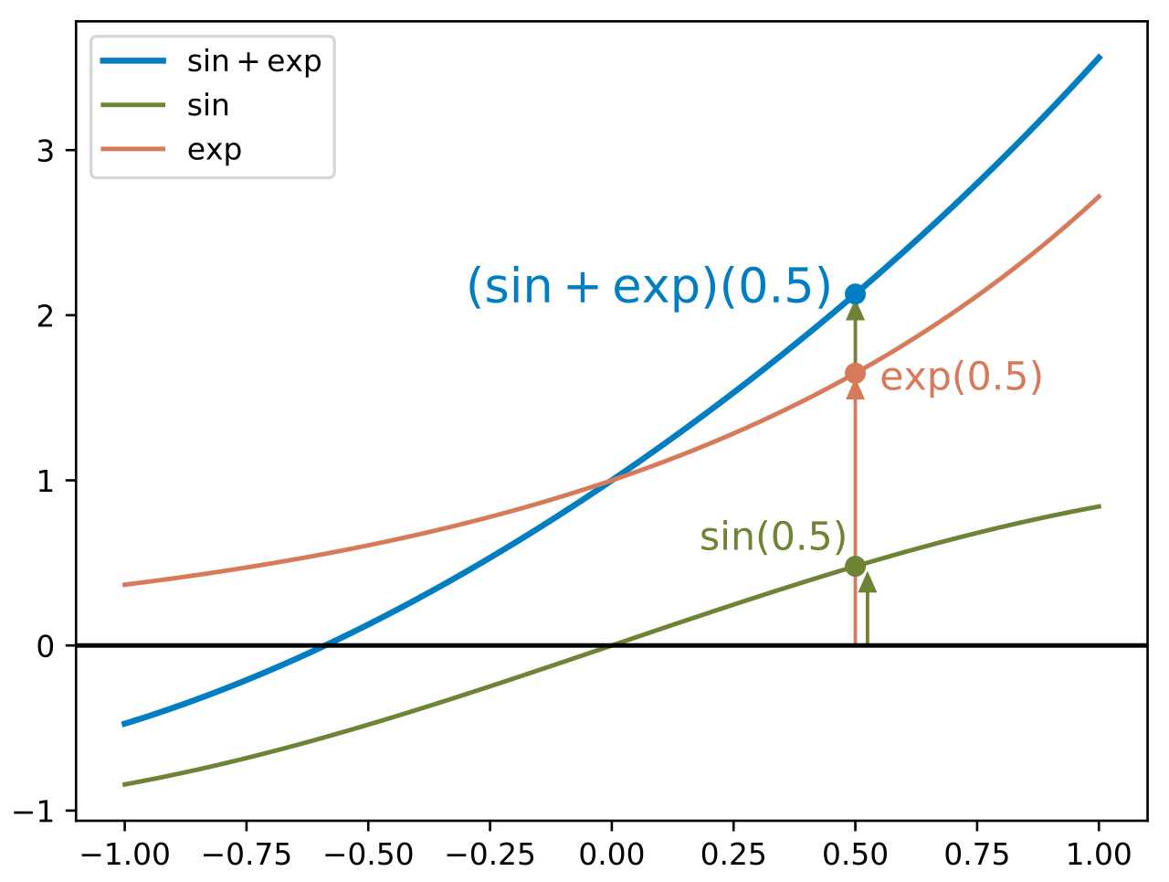
Functions from any fixed set Ω to a field F also form vector spaces, by performing addition and scalar multiplication pointwise. That is, the sum of two functions f and g is the function ${\displaystyle (f+g)}$ given by $${\displaystyle (f+g)(w)=f(w)+g(w),}$$and similarly for multiplication. Such function spaces occur in many geometric situations, when Ω is the real line or an interval, or other subsets of R. Many notions in topology and analysis, such as continuity, integrability or differentiability are well-behaved with respect to linearity: sums and scalar multiples of functions possessing such a property still have that property.^[35] Therefore, the set of such functions are vector spaces, whose study belongs to functional analysis.

Linear equations

Systems of homogeneous linear equations are closely tied to vector spaces.^[36] For example, the solutions of $${\displaystyle {\begin{alignedat}{9}&&a\,&&+\,3b\,&\,+&\,&c&\,=0\\4&&a\,&&+\,2b\,&\,+&\,2&c&\,=0\\\end{alignedat}}}$$are given by triples with arbitrary ${\displaystyle a,}$ ${\displaystyle b=a/2,}$ and ${\displaystyle c=-5a/2.}$ They form a vector space: sums and scalar multiples of such triples still satisfy the same ratios of the three variables; thus they are solutions, too. Matrices can be used to condense multiple linear equations as above into one vector equation, namely

$${\displaystyle A\mathbf {x} =\mathbf {0} ,}$$

where ${\displaystyle A={\begin{bmatrix}1&3&1\\4&2&2\end{bmatrix}}}$ is the matrix containing the coefficients of the given equations, ${\displaystyle \mathbf {x} }$ is the vector ${\displaystyle (a,b,c),}$ ${\displaystyle A\mathbf {x} }$ denotes the matrix product, and ${\displaystyle \mathbf {0} =(0,0)}$ is the zero vector. In a similar vein, the solutions of homogeneous linear differential equations form vector spaces. For example,

$${\displaystyle f^{\prime \prime }(x)+2f^{\prime }(x)+f(x)=0}$$

yields ${\displaystyle f(x)=ae^{-x}+bxe^{-x},}$ where ${\displaystyle a}$ and ${\displaystyle b}$ are arbitrary constants, and ${\displaystyle e^{x}}$ is the natural exponential function.

Linear maps and matrices

The relation of two vector spaces can be expressed by linear map or linear transformation. They are functions that reflect the vector space structure, that is, they preserve sums and scalar multiplication: $${\displaystyle {\begin{aligned}f(\mathbf {v} +\mathbf {w} )&=f(\mathbf {v} )+f(\mathbf {w} ),\\f(a\cdot \mathbf {v} )&=a\cdot f(\mathbf {v} )\end{aligned}}}$$ for all ${\displaystyle \mathbf {v} }$ and ${\displaystyle \mathbf {w} }$ in ${\displaystyle V,}$ all ${\displaystyle a}$ in ${\displaystyle F.}$^[37]

An isomorphism is a linear map f : V → W such that there exists an inverse map g : W → V, which is a map such that the two possible compositions f ∘ g : W → W and g ∘ f : V → V are identity maps. Equivalently, f is both one-to-one (injective) and onto (surjective).^[38] If there exists an isomorphism between V and W, the two spaces are said to be isomorphic; they are then essentially identical as vector spaces, since all identities holding in V are, via f, transported to similar ones in W, and vice versa via g.

Describing an arrow vector v by its coordinates x and y yields an isomorphism of vector spaces.

For example, the arrows in the plane and the ordered pairs of numbers vector spaces in the introduction above (see § Examples) are isomorphic: a planar arrow v departing at the origin of some (fixed) coordinate system can be expressed as an ordered pair by considering the x- and y-component of the arrow, as shown in the image at the right. Conversely, given a pair (x, y), the arrow going by x to the right (or to the left, if x is negative), and y up (down, if y is negative) turns back the arrow v.^[39]

Linear maps V → W between two vector spaces form a vector space Hom_F(V, W), also denoted L(V, W), or 𝓛(V, W).^[40] The space of linear maps from V to F is called the dual vector space, denoted V^∗.^[41] Via the injective natural map V → V^∗∗, any vector space can be embedded into its bidual; the map is an isomorphism if and only if the space is finite-dimensional.^[42]

Once a basis of V is chosen, linear maps f : V → W are completely determined by specifying the images of the basis vectors, because any element of V is expressed uniquely as a linear combination of them.^[43] If dim V = dim W, a 1-to-1 correspondence between fixed bases of V and W gives rise to a linear map that maps any basis element of V to the corresponding basis element of W. It is an isomorphism, by its very definition.^[44] Therefore, two vector spaces over a given field are isomorphic if their dimensions agree and vice versa. Another way to express this is that any vector space over a given field is completely classified (up to isomorphism) by its dimension, a single number. In particular, any n-dimensional F-vector space V is isomorphic to Fⁿ. However, there is no "canonical" or preferred isomorphism; an isomorphism φ : Fⁿ → V is equivalent to the choice of a basis of V, by mapping the standard basis of Fⁿ to V, via φ.

Matrices

A typical matrix

Matrices are a useful notion to encode linear maps.^[45] They are written as a rectangular array of scalars as in the image at the right. Any m-by-n matrix ${\displaystyle A}$ gives rise to a linear map from Fⁿ to F^m, by the following $${\displaystyle \mathbf {x} =(x_{1},x_{2},\ldots ,x_{n})\mapsto \left(\sum _{j=1}^{n}a_{1j}x_{j},\sum _{j=1}^{n}a_{2j}x_{j},\ldots ,\sum _{j=1}^{n}a_{mj}x_{j}\right),}$$ where ${\textstyle \sum }$ denotes summation, or by using the matrix multiplication of the matrix ${\displaystyle A}$ with the coordinate vector ${\displaystyle \mathbf {x} }$:

$${\displaystyle \mathbf {x} \mapsto A\mathbf {x} .}$$

Moreover, after choosing bases of V and W, any linear map f : V → W is uniquely represented by a matrix via this assignment.^[46]

The volume of this parallelepiped is the absolute value of the determinant of the 3-by-3 matrix formed by the vectors r₁, r₂, and r₃.

The determinant det (A) of a square matrix A is a scalar that tells whether the associated map is an isomorphism or not: to be so it is sufficient and necessary that the determinant is nonzero.^[47] The linear transformation of Rⁿ corresponding to a real n-by-n matrix is orientation preserving if and only if its determinant is positive.

Eigenvalues and eigenvectors

Endomorphisms, linear maps f : V → V, are particularly important since in this case vectors v can be compared with their image under f, f(v). Any nonzero vector v satisfying λv = f(v), where λ is a scalar, is called an eigenvector of f with eigenvalue λ.^[48] Equivalently, v is an element of the kernel of the difference f − λ · Id (where Id is the identity map V → V). If V is finite-dimensional, this can be rephrased using determinants: f having eigenvalue λ is equivalent to $${\displaystyle \det(f-\lambda \cdot \operatorname {Id} )=0.}$$By spelling out the definition of the determinant, the expression on the left hand side can be seen to be a polynomial function in λ, called the characteristic polynomial of f.^[49] If the field F is large enough to contain a zero of this polynomial (which automatically happens for F algebraically closed, such as F = C) any linear map has at least one eigenvector. The vector space V may or may not possess an eigenbasis, a basis consisting of eigenvectors. This phenomenon is governed by the Jordan canonical form of the map.^[50] The set of all eigenvectors corresponding to a particular eigenvalue of f forms a vector space known as the eigenspace corresponding to the eigenvalue (and f) in question.

Basic constructions

In addition to the above concrete examples, there are a number of standard linear algebraic constructions that yield vector spaces related to given ones.

Subspaces and quotient spaces

A line passing through the origin (blue, thick) in R3 is a linear subspace. It is the intersection of two planes (green and yellow).

A nonempty subset ${\displaystyle W}$ of a vector space ${\displaystyle V}$ that is closed under addition and scalar multiplication (and therefore contains the ${\displaystyle \mathbf {0} }$-vector of ${\displaystyle V}$) is called a linear subspace of ${\displaystyle V}$, or simply a subspace of ${\displaystyle V}$, when the ambient space is unambiguously a vector space.^{[51][nb 4]} Subspaces of ${\displaystyle V}$ are vector spaces (over the same field) in their own right. The intersection of all subspaces containing a given set ${\displaystyle S}$ of vectors is called its span, and it is the smallest subspace of ${\displaystyle V}$ containing the set ${\displaystyle S}$. Expressed in terms of elements, the span is the subspace consisting of all the linear combinations of elements of ${\displaystyle S}$.^[52]

Linear subspace of dimension 1 and 2 are referred to as a line (also vector line), and a plane respectively. If W is an n-dimensional vector space, any subspace of dimension 1 less, i.e., of dimension ${\displaystyle n-1}$ is called a hyperplane.^[53]

The counterpart to subspaces are quotient vector spaces.^[54] Given any subspace ${\displaystyle W\subseteq V}$, the quotient space ${\displaystyle V/W}$ (" ${\displaystyle V}$ modulo ${\displaystyle W}$") is defined as follows: as a set, it consists of $${\displaystyle \mathbf {v} +W=\{\mathbf {v} +\mathbf {w} :\mathbf {w} \in W\},}$$where ${\displaystyle \mathbf {v} }$ is an arbitrary vector in ${\displaystyle V}$. The sum of two such elements ${\displaystyle \mathbf {v} _{1}+W}$ and ${\displaystyle \mathbf {v} _{2}+W}$ is ${\displaystyle \left(\mathbf {v} _{1}+\mathbf {v} _{2}\right)+W}$, and scalar multiplication is given by ${\displaystyle a\cdot (\mathbf {v} +W)=(a\cdot \mathbf {v} )+W}$. The key point in this definition is that ${\displaystyle \mathbf {v} _{1}+W=\mathbf {v} _{2}+W}$ if and only if the difference of ${\displaystyle \mathbf {v} _{1}}$ and ${\displaystyle \mathbf {v} _{2}}$ lies in ${\displaystyle W}$.^{[nb 5]} This way, the quotient space "forgets" information that is contained in the subspace ${\displaystyle W}$.

The kernel ${\displaystyle \ker(f)}$ of a linear map ${\displaystyle f:V\to W}$ consists of vectors ${\displaystyle \mathbf {v} }$ that are mapped to ${\displaystyle \mathbf {0} }$ in ${\displaystyle W}$.^[55] The kernel and the image ${\displaystyle \operatorname {im} (f)=\{f(\mathbf {v} ):\mathbf {v} \in V\}}$ are subspaces of ${\displaystyle V}$ and ${\displaystyle W}$, respectively.^[56]

An important example is the kernel of a linear map ${\displaystyle \mathbf {x} \mapsto A\mathbf {x} }$ for some fixed matrix ${\displaystyle A}$. The kernel of this map is the subspace of vectors ${\displaystyle \mathbf {x} }$ such that ${\displaystyle A\mathbf {x} =\mathbf {0} }$, which is precisely the set of solutions to the system of homogeneous linear equations belonging to ${\displaystyle A}$. This concept also extends to linear differential equations $${\displaystyle a_{0}f+a_{1}{\frac {df}{dx}}+a_{2}{\frac {d^{2}f}{dx^{2}}}+\cdots +a_{n}{\frac {d^{n}f}{dx^{n}}}=0,}$$where the coefficients ${\displaystyle a_{i}}$ are functions in ${\displaystyle x,}$ too. In the corresponding map $${\displaystyle f\mapsto D(f)=\sum _{i=0}^{n}a_{i}{\frac {d^{i}f}{dx^{i}}},}$$the derivatives of the function ${\displaystyle f}$ appear linearly (as opposed to ${\displaystyle f^{\prime \prime }(x)^{2}}$, for example). Since differentiation is a linear procedure (that is, ${\displaystyle (f+g)^{\prime }=f^{\prime }+g^{\prime }}$ and ${\displaystyle (c\cdot f)^{\prime }=c\cdot f^{\prime }}$ for a constant ${\displaystyle c}$) this assignment is linear, called a linear differential operator. In particular, the solutions to the differential equation ${\displaystyle D(f)=0}$ form a vector space (over R or C).^[57]

The existence of kernels and images is part of the statement that the category of vector spaces (over a fixed field ${\displaystyle F}$) is an abelian category, that is, a corpus of mathematical objects and structure-preserving maps between them (a category) that behaves much like the category of abelian groups.^[58] Because of this, many statements such as the first isomorphism theorem (also called rank–nullity theorem in matrix-related terms) $${\displaystyle V/\ker(f)\;\equiv \;\operatorname {im} (f)}$$and the second and third isomorphism theorem can be formulated and proven in a way very similar to the corresponding statements for groups.

Direct product and direct sum

The direct product of vector spaces and the direct sum of vector spaces are two ways of combining an indexed family of vector spaces into a new vector space.

The direct product ${\displaystyle \textstyle {\prod _{i\in I}V_{i}}}$ of a family of vector spaces ${\displaystyle V_{i}}$ consists of the set of all tuples ${\displaystyle \left(\mathbf {v} _{i}\right)_{i\in I}}$, which specify for each index ${\displaystyle i}$ in some index set ${\displaystyle I}$ an element ${\displaystyle \mathbf {v} _{i}}$ of ${\displaystyle V_{i}}$.^[59] Addition and scalar multiplication is performed componentwise. A variant of this construction is the direct sum ${\textstyle \bigoplus _{i\in I}V_{i}}$ (also called coproduct and denoted ${\textstyle \coprod _{i\in I}V_{i}}$), where only tuples with finitely many nonzero vectors are allowed. If the index set ${\displaystyle I}$ is finite, the two constructions agree, but in general they are different.

Tensor product

The tensor product ${\displaystyle V\otimes _{F}W,}$ or simply ${\displaystyle V\otimes W,}$ of two vector spaces ${\displaystyle V}$ and ${\displaystyle W}$ is one of the central notions of multilinear algebra which deals with extending notions such as linear maps to several variables. A map ${\displaystyle g:V\times W\to X}$ from the Cartesian product ${\displaystyle V\times W}$ is called bilinear if ${\displaystyle g}$ is linear in both variables ${\displaystyle \mathbf {v} }$ and ${\displaystyle \mathbf {w} .}$ That is to say, for fixed ${\displaystyle \mathbf {w} }$ the map ${\displaystyle \mathbf {v} \mapsto g(\mathbf {v} ,\mathbf {w} )}$ is linear in the sense above and likewise for fixed ${\displaystyle \mathbf {v} .}$

Commutative diagram depicting the universal property of the tensor product

The tensor product is a particular vector space that is a universal recipient of bilinear maps ${\displaystyle g,}$ as follows. It is defined as the vector space consisting of finite (formal) sums of symbols called tensors $${\displaystyle \mathbf {v} _{1}\otimes \mathbf {w} _{1}+\mathbf {v} _{2}\otimes \mathbf {w} _{2}+\cdots +\mathbf {v} _{n}\otimes \mathbf {w} _{n},}$$subject to the rules^[60] $${\displaystyle {\begin{alignedat}{6}a\cdot (\mathbf {v} \otimes \mathbf {w} )~&=~(a\cdot \mathbf {v} )\otimes \mathbf {w} ~=~\mathbf {v} \otimes (a\cdot \mathbf {w} ),&&~~{\text{ where }}a{\text{ is a scalar}}\\(\mathbf {v} _{1}+\mathbf {v} _{2})\otimes \mathbf {w} ~&=~\mathbf {v} _{1}\otimes \mathbf {w} +\mathbf {v} _{2}\otimes \mathbf {w} &&\\\mathbf {v} \otimes (\mathbf {w} _{1}+\mathbf {w} _{2})~&=~\mathbf {v} \otimes \mathbf {w} _{1}+\mathbf {v} \otimes \mathbf {w} _{2}.&&\\\end{alignedat}}}$$These rules ensure that the map ${\displaystyle f}$ from the ${\displaystyle V\times W}$ to ${\displaystyle V\otimes W}$ that maps a tuple ${\displaystyle (\mathbf {v} ,\mathbf {w} )}$ to ${\displaystyle \mathbf {v} \otimes \mathbf {w} }$ is bilinear. The universality states that given any vector space ${\displaystyle X}$ and any bilinear map ${\displaystyle g:V\times W\to X,}$ there exists a unique map ${\displaystyle u,}$ shown in the diagram with a dotted arrow, whose composition with ${\displaystyle f}$ equals ${\displaystyle g:}$ ${\displaystyle u(\mathbf {v} \otimes \mathbf {w} )=g(\mathbf {v} ,\mathbf {w} ).}$^[61] This is called the universal property of the tensor product, an instance of the method—much used in advanced abstract algebra—to indirectly define objects by specifying maps from or to this object.

Vector spaces with additional structure

From the point of view of linear algebra, vector spaces are completely understood insofar as any vector space over a given field is characterized, up to isomorphism, by its dimension. However, vector spaces per se do not offer a framework to deal with the question—crucial to analysis—whether a sequence of functions converges to another function. Likewise, linear algebra is not adapted to deal with infinite series, since the addition operation allows only finitely many terms to be added. Therefore, the needs of functional analysis require considering additional structures.^[62]

A vector space may be given a partial order ${\displaystyle \,\leq ,\,}$ under which some vectors can be compared.^[63] For example, ${\displaystyle n}$-dimensional real space ${\displaystyle \mathbf {R} ^{n}}$ can be ordered by comparing its vectors componentwise. Ordered vector spaces, for example Riesz spaces, are fundamental to Lebesgue integration, which relies on the ability to express a function as a difference of two positive functions $${\displaystyle f=f^{+}-f^{-}.}$$where ${\displaystyle f^{+}}$ denotes the positive part of ${\displaystyle f}$ and ${\displaystyle f^{-}}$ the negative part.^[64]

Normed vector spaces and inner product spaces

"Measuring" vectors is done by specifying a norm, a datum which measures lengths of vectors, or by an inner product, which measures angles between vectors. Norms and inner products are denoted ${\displaystyle |\mathbf {v} |}$ and ${\displaystyle \langle \mathbf {v} ,\mathbf {w} \rangle ,}$ respectively. The datum of an inner product entails that lengths of vectors can be defined too, by defining the associated norm ${\textstyle |\mathbf {v} |:={\sqrt {\langle \mathbf {v} ,\mathbf {v} \rangle }}.}$ Vector spaces endowed with such data are known as normed vector spaces and inner product spaces, respectively.^[65]

Coordinate space ${\displaystyle F^{n}}$ can be equipped with the standard dot product: $${\displaystyle \langle \mathbf {x} ,\mathbf {y} \rangle =\mathbf {x} \cdot \mathbf {y} =x_{1}y_{1}+\cdots +x_{n}y_{n}.}$$In ${\displaystyle \mathbf {R} ^{2},}$ this reflects the common notion of the angle between two vectors ${\displaystyle \mathbf {x} }$ and ${\displaystyle \mathbf {y} ,}$ by the law of cosines: $${\displaystyle \mathbf {x} \cdot \mathbf {y} =\cos \left(\angle (\mathbf {x} ,\mathbf {y} )\right)\cdot |\mathbf {x} |\cdot |\mathbf {y} |.}$$Because of this, two vectors satisfying ${\displaystyle \langle \mathbf {x} ,\mathbf {y} \rangle =0}$ are called orthogonal. An important variant of the standard dot product is used in Minkowski space: ${\displaystyle \mathbf {R} ^{4}}$ endowed with the Lorentz product^[66] $${\displaystyle \langle \mathbf {x} |\mathbf {y} \rangle =x_{1}y_{1}+x_{2}y_{2}+x_{3}y_{3}-x_{4}y_{4}.}$$In contrast to the standard dot product, it is not positive definite: ${\displaystyle \langle \mathbf {x} |\mathbf {x} \rangle }$ also takes negative values, for example, for ${\displaystyle \mathbf {x} =(0,0,0,1).}$ Singling out the fourth coordinate—corresponding to time, as opposed to three space-dimensions—makes it useful for the mathematical treatment of special relativity.

Topological vector spaces

Convergence questions are treated by considering vector spaces ${\displaystyle V}$ carrying a compatible topology, a structure that allows one to talk about elements being close to each other.^[67] Compatible here means that addition and scalar multiplication have to be continuous maps. Roughly, if ${\displaystyle \mathbf {x} }$ and ${\displaystyle \mathbf {y} }$ in ${\displaystyle V}$, and ${\displaystyle a}$ in ${\displaystyle F}$ vary by a bounded amount, then so do ${\displaystyle \mathbf {x} +\mathbf {y} }$ and ${\displaystyle a\mathbf {x} .}$^{[nb 6]} To make sense of specifying the amount a scalar changes, the field ${\displaystyle F}$ also has to carry a topology in this context; a common choice is the reals or the complex numbers.

In such topological vector spaces one can consider series of vectors. The infinite sum $${\displaystyle \sum _{i=1}^{\infty }f_{i}~=~\lim _{n\to \infty }f_{1}+\cdots +f_{n}}$$denotes the limit of the corresponding finite partial sums of the sequence ${\displaystyle f_{1},f_{2},\ldots }$ of elements of ${\displaystyle V.}$ For example, the ${\displaystyle f_{i}}$ could be (real or complex) functions belonging to some function space ${\displaystyle V,}$ in which case the series is a function series. The mode of convergence of the series depends on the topology imposed on the function space. In such cases, pointwise convergence and uniform convergence are two prominent examples.^[68]

Unit "spheres" in ${\displaystyle \mathbf {R} ^{2}}$ consist of plane vectors of norm 1. Depicted are the unit spheres in different ${\displaystyle p}$-norms, for ${\displaystyle p=1,2,}$ and ${\displaystyle \infty .}$ The bigger diamond depicts points of 1-norm equal to 2.

A way to ensure the existence of limits of certain infinite series is to restrict attention to spaces where any Cauchy sequence has a limit; such a vector space is called complete. Roughly, a vector space is complete provided that it contains all necessary limits. For example, the vector space of polynomials on the unit interval ${\displaystyle [0,1],}$ equipped with the topology of uniform convergence is not complete because any continuous function on ${\displaystyle [0,1]}$ can be uniformly approximated by a sequence of polynomials, by the Weierstrass approximation theorem.^[69] In contrast, the space of all continuous functions on ${\displaystyle [0,1]}$ with the same topology is complete.^[70] A norm gives rise to a topology by defining that a sequence of vectors ${\displaystyle \mathbf {v} _{n}}$ converges to ${\displaystyle \mathbf {v} }$ if and only if $${\displaystyle \lim _{n\to \infty }|\mathbf {v} _{n}-\mathbf {v} |=0.}$$Banach and Hilbert spaces are complete topological vector spaces whose topologies are given, respectively, by a norm and an inner product. Their study—a key piece of functional analysis—focuses on infinite-dimensional vector spaces, since all norms on finite-dimensional topological vector spaces give rise to the same notion of convergence.^[71] The image at the right shows the equivalence of the ${\displaystyle 1}$-norm and ${\displaystyle \infty }$-norm on ${\displaystyle \mathbf {R} ^{2}:}$ as the unit "balls" enclose each other, a sequence converges to zero in one norm if and only if it so does in the other norm. In the infinite-dimensional case, however, there will generally be inequivalent topologies, which makes the study of topological vector spaces richer than that of vector spaces without additional data.

From a conceptual point of view, all notions related to topological vector spaces should match the topology. For example, instead of considering all linear maps (also called functionals) ${\displaystyle V\to W,}$ maps between topological vector spaces are required to be continuous.^[72] In particular, the (topological) dual space ${\displaystyle V^{*}}$ consists of continuous functionals ${\displaystyle V\to \mathbf {R} }$ (or to ${\displaystyle \mathbf {C} }$). The fundamental Hahn–Banach theorem is concerned with separating subspaces of appropriate topological vector spaces by continuous functionals.^[73]

Banach spaces

Banach spaces, introduced by Stefan Banach, are complete normed vector spaces.^[74]

A first example is the vector space ${\displaystyle \ell ^{p}}$ consisting of infinite vectors with real entries ${\displaystyle \mathbf {x} =\left(x_{1},x_{2},\ldots ,x_{n},\ldots \right)}$whose ${\displaystyle p}$-norm ${\displaystyle (1\leq p\leq \infty )}$ given by $${\displaystyle \|\mathbf {x} \|_{\infty }:=\sup _{i}|x_{i}|\qquad {\text{ for }}p=\infty ,{\text{ and }}}$$ $${\displaystyle \|\mathbf {x} \|_{p}:=\left(\sum _{i}|x_{i}|^{p}\right)^{\frac {1}{p}}\qquad {\text{ for }}p<\infty .}$$

The topologies on the infinite-dimensional space ${\displaystyle \ell ^{p}}$ are inequivalent for different ${\displaystyle p.}$ For example, the sequence of vectors ${\displaystyle \mathbf {x} _{n}=\left(2^{-n},2^{-n},\ldots ,2^{-n},0,0,\ldots \right),}$ in which the first ${\displaystyle 2^{n}}$ components are ${\displaystyle 2^{-n}}$ and the following ones are ${\displaystyle 0,}$ converges to the zero vector for ${\displaystyle p=\infty ,}$ but does not for ${\displaystyle p=1:}$ $${\displaystyle \|\mathbf {x} _{n}\|_{\infty }=\sup(2^{-n},0)=2^{-n}\to 0,}$$ but $${\displaystyle \|\mathbf {x} _{n}\|_{1}=\sum _{i=1}^{2^{n}}2^{-n}=2^{n}\cdot 2^{-n}=1.}$$

More generally than sequences of real numbers, functions ${\displaystyle f:\Omega \to \mathbb {R} }$ are endowed with a norm that replaces the above sum by the Lebesgue integral $${\displaystyle \|f\|_{p}:=\left(\int _{\Omega }|f(x)|^{p}\,{d\mu (x)}\right)^{\frac {1}{p}}.}$$

The space of integrable functions on a given domain ${\displaystyle \Omega }$ (for example an interval) satisfying ${\displaystyle \|f\|_{p}<\infty ,}$ and equipped with this norm are called Lebesgue spaces, denoted ${\displaystyle L^{\;\!p}(\Omega ).}$^{[nb 7]}

These spaces are complete.^[75] (If one uses the Riemann integral instead, the space is not complete, which may be seen as a justification for Lebesgue's integration theory.^{[nb 8]}) Concretely this means that for any sequence of Lebesgue-integrable functions ${\displaystyle f_{1},f_{2},\ldots ,f_{n},\ldots }$ with ${\displaystyle \|f_{n}\|_{p}<\infty ,}$ satisfying the condition $${\displaystyle \lim _{k,\ n\to \infty }\int _{\Omega }\left|f_{k}(x)-f_{n}(x)\right|^{p}\,{d\mu (x)}=0}$$there exists a function ${\displaystyle f(x)}$ belonging to the vector space ${\displaystyle L^{\;\!p}(\Omega )}$ such that $${\displaystyle \lim _{k\to \infty }\int _{\Omega }\left|f(x)-f_{k}(x)\right|^{p}\,{d\mu (x)}=0.}$$

Imposing boundedness conditions not only on the function, but also on its derivatives leads to Sobolev spaces.^[76]

Hilbert spaces

The succeeding snapshots show summation of 1 to 5 terms in approximating a periodic function (blue) by finite sum of sine functions (red).

Complete inner product spaces are known as Hilbert spaces, in honor of David Hilbert.^[77] The Hilbert space ${\displaystyle L^{2}(\Omega ),}$ with inner product given by $${\displaystyle \langle f\ ,\ g\rangle =\int _{\Omega }f(x){\overline {g(x)}}\,dx,}$$where ${\displaystyle {\overline {g(x)}}}$ denotes the complex conjugate of ${\displaystyle g(x),}$^{[78][nb 9]} is a key case.

By definition, in a Hilbert space, any Cauchy sequence converges to a limit. Conversely, finding a sequence of functions ${\displaystyle f_{n}}$ with desirable properties that approximate a given limit function is equally crucial. Early analysis, in the guise of the Taylor approximation, established an approximation of differentiable functions ${\displaystyle f}$ by polynomials.^[79] By the Stone–Weierstrass theorem, every continuous function on ${\displaystyle [a,b]}$ can be approximated as closely as desired by a polynomial.^[80] A similar approximation technique by trigonometric functions is commonly called Fourier expansion, and is much applied in engineering. More generally, and more conceptually, the theorem yields a simple description of what "basic functions", or, in abstract Hilbert spaces, what basic vectors suffice to generate a Hilbert space ${\displaystyle H,}$ in the sense that the closure of their span (that is, finite linear combinations and limits of those) is the whole space. Such a set of functions is called a basis of ${\displaystyle H,}$ its cardinality is known as the Hilbert space dimension.^{[nb 10]} Not only does the theorem exhibit suitable basis functions as sufficient for approximation purposes, but also together with the Gram–Schmidt process, it enables one to construct a basis of orthogonal vectors.^[81] Such orthogonal bases are the Hilbert space generalization of the coordinate axes in finite-dimensional Euclidean space.

The solutions to various differential equations can be interpreted in terms of Hilbert spaces. For example, a great many fields in physics and engineering lead to such equations, and frequently solutions with particular physical properties are used as basis functions, often orthogonal.^[82] As an example from physics, the time-dependent Schrödinger equation in quantum mechanics describes the change of physical properties in time by means of a partial differential equation, whose solutions are called wavefunctions.^[83] Definite values for physical properties such as energy, or momentum, correspond to eigenvalues of a certain (linear) differential operator and the associated wavefunctions are called eigenstates. The spectral theorem decomposes a linear compact operator acting on functions in terms of these eigenfunctions and their eigenvalues.^[84]

Algebras over fields

A hyperbola, given by the equation ${\displaystyle x\cdot y=1.}$ The coordinate ring of functions on this hyperbola is given by ${\displaystyle \mathbf {R} [x,y]/(x\cdot y-1),}$ an infinite-dimensional vector space over ${\displaystyle \mathbf {R} .}$

General vector spaces do not possess a multiplication between vectors. A vector space equipped with an additional bilinear operator defining the multiplication of two vectors is an algebra over a field (or F-algebra if the field F is specified).^[85]

For example, the set of all polynomials ${\displaystyle p(t)}$ forms an algebra known as the polynomial ring: using that the sum of two polynomials is a polynomial, they form a vector space; they form an algebra since the product of two polynomials is again a polynomial. Rings of polynomials (in several variables) and their quotients form the basis of algebraic geometry, because they are rings of functions of algebraic geometric objects.^[86]

Another crucial example are Lie algebras, which are neither commutative nor associative, but the failure to be so is limited by the constraints ( ${\displaystyle [x,y]}$ denotes the product of ${\displaystyle x}$ and ${\displaystyle y}$):

• ${\displaystyle [x,y]=-[y,x]}$ (anticommutativity), and
• ${\displaystyle [x,[y,z]]+[y,[z,x]]+[z,[x,y]]=0}$ (Jacobi identity).^[87]

Examples include the vector space of ${\displaystyle n}$-by- ${\displaystyle n}$ matrices, with ${\displaystyle [x,y]=xy-yx,}$ the commutator of two matrices, and ${\displaystyle \mathbf {R} ^{3},}$ endowed with the cross product.

The tensor algebra ${\displaystyle \operatorname {T} (V)}$ is a formal way of adding products to any vector space ${\displaystyle V}$ to obtain an algebra.^[88] As a vector space, it is spanned by symbols, called simple tensors $${\displaystyle \mathbf {v} _{1}\otimes \mathbf {v} _{2}\otimes \cdots \otimes \mathbf {v} _{n},}$$where the degree ${\displaystyle n}$ varies. The multiplication is given by concatenating such symbols, imposing the distributive law under addition, and requiring that scalar multiplication commute with the tensor product ⊗, much the same way as with the tensor product of two vector spaces introduced in the above section on tensor products. In general, there are no relations between ${\displaystyle \mathbf {v} _{1}\otimes \mathbf {v} _{2}}$ and ${\displaystyle \mathbf {v} _{2}\otimes \mathbf {v} _{1}.}$ Forcing two such elements to be equal leads to the symmetric algebra, whereas forcing ${\displaystyle \mathbf {v} _{1}\otimes \mathbf {v} _{2}=-\mathbf {v} _{2}\otimes \mathbf {v} _{1}}$ yields the exterior algebra.^[89]

Related structures

Vector bundles

A Möbius strip. Locally, it looks like U × R.

A vector bundle is a family of vector spaces parametrized continuously by a topological space X.^[90] More precisely, a vector bundle over X is a topological space E equipped with a continuous map $${\displaystyle \pi :E\to X}$$such that for every x in X, the fiber π⁻¹(x) is a vector space. The case dim V = 1 is called a line bundle. For any vector space V, the projection X × V → X makes the product X × V into a "trivial" vector bundle. Vector bundles over X are required to be locally a product of X and some (fixed) vector space V: for every x in X, there is a neighborhood U of x such that the restriction of π to π⁻¹(U) is isomorphic^{[nb 11]} to the trivial bundle U × V → U. Despite their locally trivial character, vector bundles may (depending on the shape of the underlying space X) be "twisted" in the large (that is, the bundle need not be (globally isomorphic to) the trivial bundle X × V). For example, the Möbius strip can be seen as a line bundle over the circle S¹ (by identifying open intervals with the real line). It is, however, different from the cylinder S¹ × R, because the latter is orientable whereas the former is not.^[91]

Properties of certain vector bundles provide information about the underlying topological space. For example, the tangent bundle consists of the collection of tangent spaces parametrized by the points of a differentiable manifold. The tangent bundle of the circle S¹ is globally isomorphic to S¹ × R, since there is a global nonzero vector field on S¹.^{[nb 12]} In contrast, by the hairy ball theorem, there is no (tangent) vector field on the 2-sphere S² which is everywhere nonzero.^[92] K-theory studies the isomorphism classes of all vector bundles over some topological space.^[93] In addition to deepening topological and geometrical insight, it has purely algebraic consequences, such as the classification of finite-dimensional real division algebras: R, C, the quaternions H and the octonions O.

The cotangent bundle of a differentiable manifold consists, at every point of the manifold, of the dual of the tangent space, the cotangent space. Sections of that bundle are known as differential one-forms.

Modules

Modules are to rings what vector spaces are to fields: the same axioms, applied to a ring R instead of a field F, yield modules.^[94] The theory of modules, compared to that of vector spaces, is complicated by the presence of ring elements that do not have multiplicative inverses. For example, modules need not have bases, as the Z-module (that is, abelian group) Z/2Z shows; those modules that do (including all vector spaces) are known as free modules. Nevertheless, a vector space can be compactly defined as a module over a ring which is a field, with the elements being called vectors. Some authors use the term vector space to mean modules over a division ring.^[95] The algebro-geometric interpretation of commutative rings via their spectrum allows the development of concepts such as locally free modules, the algebraic counterpart to vector bundles.

Affine and projective spaces

An affine plane (light blue) in R³. It is a two-dimensional subspace shifted by a vector x (red).

Roughly, affine spaces are vector spaces whose origins are not specified.^[96] More precisely, an affine space is a set with a free transitive vector space action. In particular, a vector space is an affine space over itself, by the map $${\displaystyle V\times V\to W,\;(\mathbf {v} ,\mathbf {a} )\mapsto \mathbf {a} +\mathbf {v} .}$$If W is a vector space, then an affine subspace is a subset of W obtained by translating a linear subspace V by a fixed vector x ∈ W; this space is denoted by x + V (it is a coset of V in W) and consists of all vectors of the form x + v for v ∈ V. An important example is the space of solutions of a system of inhomogeneous linear equations $${\displaystyle A\mathbf {v} =\mathbf {b} }$$generalizing the homogeneous case discussed in the above section on linear equations, which can be found by setting ${\displaystyle \mathbf {b} =\mathbf {0} }$ in this equation.^[97] The space of solutions is the affine subspace x + V where x is a particular solution of the equation, and V is the space of solutions of the homogeneous equation (the nullspace of A).

The set of one-dimensional subspaces of a fixed finite-dimensional vector space V is known as projective space; it may be used to formalize the idea of parallel lines intersecting at infinity.^[98] Grassmannians and flag manifolds generalize this by parametrizing linear subspaces of fixed dimension k and flags of subspaces, respectively.

Notes

1. It is also common, especially in physics, to denote vectors with an arrow on top: ${\displaystyle {\vec {v}}.}$ It is also common, especially in higher mathematics, to not use any typographical method for distinguishing vectors from other mathematical objects.
2. Scalar multiplication is not to be confused with the scalar product, which is an additional operation on some specific vector spaces, called inner product spaces. Scalar multiplication is the multiplication of a vector by a scalar that produces a vector, while the scalar product is a multiplication of two vectors that produces a scalar.
3. This axiom is not an associative property, since it refers to two different operations, scalar multiplication and field multiplication. So, it is independent from the associativity of field multiplication, which is assumed by field axioms.
4. This is typically the case when a vector space is also considered as an affine space. In this case, a linear subspace contains the zero vector, while an affine subspace does not necessarily contain it.
5. Some authors, such as Roman (2005), choose to start with this equivalence relation and derive the concrete shape of ${\displaystyle V/W}$ from this.
6. This requirement implies that the topology gives rise to a uniform structure, Bourbaki (1989), loc = ch. II.
7. The triangle inequality for ${\displaystyle \|f+g\|_{p}\leq \|f\|_{p}+\|g\|_{p}}$ is provided by the Minkowski inequality. For technical reasons, in the context of functions one has to identify functions that agree almost everywhere to get a norm, and not only a seminorm.
8. "Many functions in ${\displaystyle L^{2}}$ of Lebesgue measure, being unbounded, cannot be integrated with the classical Riemann integral. So spaces of Riemann integrable functions would not be complete in the ${\displaystyle L^{2}}$ norm, and the orthogonal decomposition would not apply to them. This shows one of the advantages of Lebesgue integration.", Dudley (1989), §5.3, p. 125.
9. For ${\displaystyle p\neq 2,}$ ${\displaystyle L^{p}(\Omega )}$ is not a Hilbert space.
10. A basis of a Hilbert space is not the same thing as a basis of a linear algebra. For distinction, a linear algebra basis for a Hilbert space is called a Hamel basis.
11. That is, there is a homeomorphism from π⁻¹(U) to V × U which restricts to linear isomorphisms between fibers.
12. A line bundle, such as the tangent bundle of S¹ is trivial if and only if there is a section that vanishes nowhere, see Husemoller (1994), Corollary 8.3. The sections of the tangent bundle are just vector fields.

Citations

1. Lang 2002.
2. Brown 1991, p. 86.
3. Roman 2005, ch. 1, p. 27.
4. Brown 1991, p. 87.
5. Springer 2000, p. 185; Brown 1991, p. 86.
6. Atiyah & Macdonald 1969, p. 17.
7. Bourbaki 1998, §1.1, Definition 2.
8. Brown 1991, p. 94.
9. Brown 1991, pp. 99–101.
10. Brown 1991, p. 92.
11. Stoll & Wong 1968, p. 14.
12. Roman 2005, pp. 41–42.
13. Lang 1987, p. 10–11; Anton & Rorres 2010, p. 212.
14. Blass 1984.
15. Joshi 1989, p. 450.
16. Heil 2011, p. 126.
17. Halmos 1948, p. 12.
18. Bourbaki 1969, ch. "Algèbre linéaire et algèbre multilinéaire", pp. 78–91.
19. Bolzano 1804.
20. Möbius 1827.
21. Bellavitis 1833.
22. Dorier 1995.
23. Hamilton 1853.
24. Grassmann 2000.
25. Peano 1888, ch. IX.
26. Guo 2021.
27. Moore 1995, pp. 268–271.
28. Banach 1922.
29. Dorier 1995; Moore 1995.
30. Kreyszig 2020, p. 355.
31. Kreyszig 2020, p. 358–359.
32. Jain 2001, p. 11.
33. Lang 1987, ch. I.1.
34. Lang 2002, ch. V.1.
35. Lang 1993, ch. XII.3., p. 335.
36. Lang 1987, ch. VI.3..
37. Roman 2005, ch. 2, p. 45.
38. Lang 1987, ch. IV.4, Corollary, p. 106.
39. Nicholson 2018, ch. 7.3.
40. Lang 1987, Example IV.2.6.
41. Lang 1987, ch. VI.6.
42. Halmos 1974, p. 28, Ex. 9.
43. Lang 1987, Theorem IV.2.1, p. 95.
44. Roman 2005, Th. 2.5 and 2.6, p. 49.
45. Lang 1987, ch. V.1.
46. Lang 1987, ch. V.3., Corollary, p. 106.
47. Lang 1987, Theorem VII.9.8, p. 198.
48. Roman 2005, ch. 8, p. 135–156.
49. & Lang 1987, ch. IX.4.
50. Roman 2005, ch. 8, p. 140.
51. Roman 2005, ch. 1, p. 29.
52. Roman 2005, ch. 1, p. 35.
53. Nicholson 2018, ch. 10.4.
54. Roman 2005, ch. 3, p. 64.
55. Lang 1987, ch. IV.3..
56. Roman 2005, ch. 2, p. 48.
57. Nicholson 2018, ch. 7.4.
58. Mac Lane 1998.
59. Roman 2005, ch. 1, pp. 31–32.
60. Lang 2002, ch. XVI.1.
61. Roman (2005), Th. 14.3. See also Yoneda lemma.
62. Rudin 1991, p.3.
63. Schaefer & Wolff 1999, pp. 204–205.
64. Bourbaki 2004, ch. 2, p. 48.
65. Roman 2005, ch. 9.
66. Naber 2003, ch. 1.2.
67. Treves 1967; Bourbaki 1987.
68. Schaefer & Wolff 1999, p. 7.
69. Kreyszig 1989, §4.11-5
70. Kreyszig 1989, §1.5-5
71. Choquet 1966, Proposition III.7.2.
72. Treves 1967, p. 34–36.
73. Lang 1983, Cor. 4.1.2, p. 69.
74. Treves 1967, ch. 11.
75. Treves 1967, Theorem 11.2, p. 102.
76. Evans 1998, ch. 5.
77. Treves 1967, ch. 12.
78. Dennery & Krzywicki 1996, p.190.
79. Lang 1993, Th. XIII.6, p. 349.
80. Lang 1993, Th. III.1.1.
81. Choquet 1966, Lemma III.16.11.
82. Kreyszig 1999, Chapter 11.
83. Griffiths 1995, Chapter 1.
84. Lang 1993, ch. XVII.3.
85. Lang 2002, ch. III.1, p. 121.
86. Eisenbud 1995, ch. 1.6.
87. Varadarajan 1974.
88. Lang 2002, ch. XVI.7.
89. Lang 2002, ch. XVI.8.
90. Spivak 1999, ch. 3.
91. Kreyszig 1991, §34, p. 108.
92. Eisenberg & Guy 1979.
93. Atiyah 1989.
94. Artin 1991, ch. 12.
95. Grillet 2007.
96. Meyer 2000, Example 5.13.5, p. 436.
97. Meyer 2000, Exercise 5.13.15–17, p. 442.
98. Coxeter 1987.

References

Algebra

• Anton, Howard; Rorres, Chris (2010), Elementary Linear Algebra: Applications Version (10th ed.), John Wiley & Sons
• Artin, Michael (1991), Algebra, Prentice Hall, ISBN 978-0-89871-510-1
• Brown, William A. (1991), Matrices and vector spaces, New York: M. Dekker, ISBN 978-0-8247-8419-5
• Grillet, Pierre Antoine (2007), Abstract algebra, vol. 242, Springer Science & Business Media, doi:10.1007/978-0-387-71568-1, ISBN 978-0-387-71568-1
• Halmos, Paul R. (1948), Finite Dimensional Vector Spaces, vol. 7, Princeton University Press
• Heil, Christopher (2011), A Basis Theory Primer: Expanded Edition, Applied and Numerical Harmonic Analysis, Birkhäuser, doi:10.1007/978-0-8176-4687-5, ISBN 978-0-8176-4687-5
• Jain, M. C. (2001), Vector Spaces and Matrices in Physics, CRC Press, ISBN 978-0-8493-0978-6
• Joshi, K. D. (1989), Foundations of Discrete Mathematics, John Wiley & Sons
• Kreyszig, Erwin (2020), Advanced Engineering Mathematics, John Wiley & Sons, ISBN 978-1-119-45592-9
• Lang, Serge (1987), Linear algebra, Undergraduate Texts in Mathematics (3rd ed.), Springer, doi:10.1007/978-1-4757-1949-9, ISBN 978-1-4757-1949-9
• Lang, Serge (2002), Algebra, Graduate Texts in Mathematics, vol. 211 (Revised third ed.), New York: Springer-Verlag, ISBN 978-0-387-95385-4, MR 1878556
• Mac Lane, Saunders (1999), Algebra (3rd ed.), American Mathematical Soc., pp. 193–222, ISBN 978-0-8218-1646-2
• Meyer, Carl D. (2000), Matrix Analysis and Applied Linear Algebra, SIAM, ISBN 978-0-89871-454-8
• Nicholson, W. Keith (2018), Linear Algebra with Applications, Lyryx
• Roman, Steven (2005), Advanced Linear Algebra, Graduate Texts in Mathematics, vol. 135 (2nd ed.), Berlin, New York: Springer-Verlag, ISBN 978-0-387-24766-3
• Spindler, Karlheinz (1993), Abstract Algebra with Applications: Volume 1: Vector spaces and groups, CRC, ISBN 978-0-8247-9144-5
• Springer, T.A. (2000), Linear Algebraic Groups, Springer, ISBN 978-0-8176-4840-4
• Stoll, R. R.; Wong, E. T. (1968), Linear Algebra, Academic Press
• van der Waerden, Bartel Leendert (1993), Algebra (in German) (9th ed.), Berlin, New York: Springer-Verlag, ISBN 978-3-540-56799-8

Analysis

• Bourbaki, Nicolas (1987), Topological vector spaces, Elements of mathematics, Berlin, New York: Springer-Verlag, ISBN 978-3-540-13627-9
• Bourbaki, Nicolas (2004), Integration I, Berlin, New York: Springer-Verlag, ISBN 978-3-540-41129-1
• Braun, Martin (1993), Differential equations and their applications: an introduction to applied mathematics, Berlin, New York: Springer-Verlag, ISBN 978-0-387-97894-9
• BSE-3 (2001) [1994], "Tangent plane", Encyclopedia of Mathematics, EMS Press
• Choquet, Gustave (1966), Topology, Boston, MA: Academic Press
• Dennery, Philippe; Krzywicki, Andre (1996), Mathematics for Physicists, Courier Dover Publications, ISBN 978-0-486-69193-0
• Dudley, Richard M. (1989), Real analysis and probability, The Wadsworth & Brooks/Cole Mathematics Series, Pacific Grove, CA: Wadsworth & Brooks/Cole Advanced Books & Software, ISBN 978-0-534-10050-6
• Dunham, William (2005), The Calculus Gallery, Princeton University Press, ISBN 978-0-691-09565-3
• Evans, Lawrence C. (1998), Partial differential equations, Providence, R.I.: American Mathematical Society, ISBN 978-0-8218-0772-9
• Folland, Gerald B. (1992), Fourier Analysis and Its Applications, Brooks-Cole, ISBN 978-0-534-17094-3
• Gasquet, Claude; Witomski, Patrick (1999), Fourier Analysis and Applications: Filtering, Numerical Computation, Wavelets, Texts in Applied Mathematics, New York: Springer-Verlag, ISBN 978-0-387-98485-8
• Ifeachor, Emmanuel C.; Jervis, Barrie W. (2001), Digital Signal Processing: A Practical Approach (2nd ed.), Harlow, Essex, England: Prentice-Hall (published 2002), ISBN 978-0-201-59619-9
• Krantz, Steven G. (1999), A Panorama of Harmonic Analysis, Carus Mathematical Monographs, Washington, DC: Mathematical Association of America, ISBN 978-0-88385-031-2
• Kreyszig, Erwin (1988), Advanced Engineering Mathematics (6th ed.), New York: John Wiley & Sons, ISBN 978-0-471-85824-9
• Kreyszig, Erwin (1989), Introductory functional analysis with applications, Wiley Classics Library, New York: John Wiley & Sons, ISBN 978-0-471-50459-7, MR 0992618
• Lang, Serge (1983), Real analysis, Addison-Wesley, ISBN 978-0-201-14179-5
• Lang, Serge (1993), Real and functional analysis, Berlin, New York: Springer-Verlag, ISBN 978-0-387-94001-4
• Loomis, Lynn H. (2011) [1953], An introduction to abstract harmonic analysis, Dover, hdl:2027/uc1.b4250788, ISBN 978-0-486-48123-4, OCLC 702357363
• Narici, Lawrence; Beckenstein, Edward (2011). Topological Vector Spaces. Pure and applied mathematics (Second ed.). Boca Raton, FL: CRC Press. ISBN 978-1584888666. OCLC 144216834.
• Rudin, Walter (1991), Functional analysis (2 ed.), McGraw-Hill, ISBN 0070542368
• Schaefer, Helmut H.; Wolff, Manfred P. (1999). Topological Vector Spaces. GTM. Vol. 8 (Second ed.). New York, NY: Springer New York Imprint Springer. ISBN 978-1-4612-7155-0. OCLC 840278135.
• Treves, François (1967), Topological vector spaces, distributions and kernels, Boston, MA: Academic Press

Historical references

• Banach, Stefan (1922), "Sur les opérations dans les ensembles abstraits et leur application aux équations intégrales (On operations in abstract sets and their application to integral equations)" (PDF), Fundamenta Mathematicae (in French), 3: 133–181, doi:10.4064/fm-3-1-133-181, ISSN 0016-2736
• Bolzano, Bernard (1804), Betrachtungen über einige Gegenstände der Elementargeometrie (Considerations of some aspects of elementary geometry) (in German)
• Bellavitis, Giuso (1833), "Sopra alcune applicazioni di un nuovo metodo di geometria analitica", Il poligrafo giornale di scienze, lettre ed arti, 13, Verona: 53–61.
• Bourbaki, Nicolas (1969), Éléments d'histoire des mathématiques (Elements of history of mathematics) (in French), Paris: Hermann
• Dorier, Jean-Luc (1995), "A general outline of the genesis of vector space theory", Historia Mathematica, 22 (3): 227–261, doi:10.1006/hmat.1995.1024, MR 1347828
• Fourier, Jean Baptiste Joseph (1822), Théorie analytique de la chaleur (in French), Chez Firmin Didot, père et fils
• Grassmann, Hermann (1844), Die Lineale Ausdehnungslehre - Ein neuer Zweig der Mathematik (in German), O. Wigand, reprint: Grassmann, Hermann (2000), Kannenberg, L.C. (ed.), Extension Theory, translated by Kannenberg, Lloyd C., Providence, R.I.: American Mathematical Society, ISBN 978-0-8218-2031-5
• Guo, Hongyu (2021-06-16), What Are Tensors Exactly?, World Scientific, ISBN 978-981-12-4103-1
• Hamilton, William Rowan (1853), Lectures on Quaternions, Royal Irish Academy
• Möbius, August Ferdinand (1827), Der Barycentrische Calcul : ein neues Hülfsmittel zur analytischen Behandlung der Geometrie (Barycentric calculus: a new utility for an analytic treatment of geometry) (in German), archived from the original on 2006-11-23
• Moore, Gregory H. (1995), "The axiomatization of linear algebra: 1875–1940", Historia Mathematica, 22 (3): 262–303, doi:10.1006/hmat.1995.1025
• Peano, Giuseppe (1888), Calcolo Geometrico secondo l'Ausdehnungslehre di H. Grassmann preceduto dalle Operazioni della Logica Deduttiva (in Italian), Turin{{citation}}: CS1 maint: location missing publisher (link)
• Peano, G. (1901) Formulario mathematico: vct axioms via Internet Archive

Further references

• Ashcroft, Neil; Mermin, N. David (1976), Solid State Physics, Toronto: Thomson Learning, ISBN 978-0-03-083993-1
• Atiyah, Michael Francis (1989), K-theory, Advanced Book Classics (2nd ed.), Addison-Wesley, ISBN 978-0-201-09394-0, MR 1043170
• Atiyah, Michael Francis; Macdonald, Ian Grant (1969), Introduction to Commutative Algebra, Advanced Book Classics, Addison-Wesley
• Blass, Andreas (1984), "Existence of bases implies the axiom of choice" (PDF), Axiomatic set theory, Contemporary Mathematics volume 31, Providence, R.I.: American Mathematical Society, pp. 31–33, ISBN 978-0-8218-5026-8, MR 0763890
• Bourbaki, Nicolas (1998), Elements of Mathematics : Algebra I Chapters 1-3, Berlin, New York: Springer-Verlag, ISBN 978-3-540-64243-5
• Bourbaki, Nicolas (1989), General Topology. Chapters 1-4, Berlin, New York: Springer-Verlag, ISBN 978-3-540-64241-1
• Coxeter, Harold Scott MacDonald (1987), Projective Geometry (2nd ed.), Berlin, New York: Springer-Verlag, ISBN 978-0-387-96532-1
• Eisenberg, Murray; Guy, Robert (1979), "A proof of the hairy ball theorem", The American Mathematical Monthly, 86 (7): 572–574, doi:10.2307/2320587, JSTOR 2320587
• Eisenbud, David (1995), Commutative algebra, Graduate Texts in Mathematics, vol. 150, Berlin, New York: Springer-Verlag, ISBN 978-0-387-94269-8, MR 1322960
• Goldrei, Derek (1996), Classic Set Theory: A guided independent study (1st ed.), London: Chapman and Hall, ISBN 978-0-412-60610-6
• Griffiths, David J. (1995), Introduction to Quantum Mechanics, Upper Saddle River, NJ: Prentice Hall, ISBN 978-0-13-124405-4
• Halmos, Paul R. (1974), Finite-dimensional vector spaces, Berlin, New York: Springer-Verlag, ISBN 978-0-387-90093-3
• Halpern, James D. (Jun 1966), "Bases in Vector Spaces and the Axiom of Choice", Proceedings of the American Mathematical Society, 17 (3): 670–673, doi:10.2307/2035388, JSTOR 2035388
• Hughes-Hallett, Deborah; McCallum, William G.; Gleason, Andrew M. (2013), Calculus : Single and Multivariable (6 ed.), John Wiley & Sons, ISBN 978-0470-88861-2
• Husemoller, Dale (1994), Fibre Bundles (3rd ed.), Berlin, New York: Springer-Verlag, ISBN 978-0-387-94087-8
• Jost, Jürgen (2005), Riemannian Geometry and Geometric Analysis (4th ed.), Berlin, New York: Springer-Verlag, ISBN 978-3-540-25907-7
• Kreyszig, Erwin (1991), Differential geometry, New York: Dover Publications, pp. xiv+352, ISBN 978-0-486-66721-8
• Kreyszig, Erwin (1999), Advanced Engineering Mathematics (8th ed.), New York: John Wiley & Sons, ISBN 978-0-471-15496-9
• Luenberger, David (1997), Optimization by vector space methods, New York: John Wiley & Sons, ISBN 978-0-471-18117-0
• Mac Lane, Saunders (1998), Categories for the Working Mathematician (2nd ed.), Berlin, New York: Springer-Verlag, ISBN 978-0-387-98403-2
• Misner, Charles W.; Thorne, Kip; Wheeler, John Archibald (1973), Gravitation, W. H. Freeman, ISBN 978-0-7167-0344-0
• Naber, Gregory L. (2003), The geometry of Minkowski spacetime, New York: Dover Publications, ISBN 978-0-486-43235-9, MR 2044239
• Schönhage, A.; Strassen, Volker (1971), "Schnelle Multiplikation großer Zahlen (Fast multiplication of big numbers)", Computing (in German), 7 (3–4): 281–292, doi:10.1007/bf02242355, ISSN 0010-485X, S2CID 9738629
• Spivak, Michael (1999), A Comprehensive Introduction to Differential Geometry (Volume Two), Houston, TX: Publish or Perish
• Stewart, Ian (1975), Galois Theory, Chapman and Hall Mathematics Series, London: Chapman and Hall, ISBN 978-0-412-10800-6
• Varadarajan, V. S. (1974), Lie groups, Lie algebras, and their representations, Prentice Hall, ISBN 978-0-13-535732-3
• Wallace, G.K. (Feb 1992), "The JPEG still picture compression standard" (PDF), IEEE Transactions on Consumer Electronics, 38 (1): xviii–xxxiv, CiteSeerX 10.1.1.318.4292, doi:10.1109/30.125072, ISSN 0098-3063, archived from the original (PDF) on 2007-01-13, retrieved 2017-10-25
• Weibel, Charles A. (1994). An introduction to homological algebra. Cambridge Studies in Advanced Mathematics. Vol. 38. Cambridge University Press. ISBN 978-0-521-55987-4. MR 1269324. OCLC 36131259.

External links

• "Vector space", Encyclopedia of Mathematics, EMS Press, 2001 [1994]